This post is an excerpt from my Master’s Thesis, which explains the formal tone and the use of the editorial “we”.
An often ignored aspect of sky and atmosphere rendering is the strong wavelength dependency of the atmospheric medium. This is caused by the optical properties of both molecular scatterers and ozone being highly variable depending on the wavelength of light interacting with them. To take this relationship into account in a light transport simulation, offline renderers usually resort to uniform spectral sampling or more elaborated spectral sampling methods like Hero Wavelength Sampling, while real-time renderers often choose to completely ignore this behaviour and perform traditional RGB rendering.
In uniform spectral sampling, we pick \(n_\lambda\) uniformly distributed samples in a portion of the electromagnetic spectrum (usually the visible spectrum). For each pixel in the rendered image, \(n_\lambda\) rays are fired from the camera, each with an associated wavelength, making all the interactions between the rays and the scene wavelength-dependent. Consequently, compared to traditional RGB rendering, spectral rendering requires substantially more data to represent the optical properties of the scene, which can be challenging to obtain in most cases. Luckily, in the case of the atmosphere of Earth, there is plenty of available data thanks to atmospheric sciences research.
Spectral rendering can sometimes offer more accurate results since it is able to capture optical phenomena that would otherwise be impossible to recreate, like iridescence. However, spectral rendering is quite sensitive to which portion of the electromagnetic spectrum is used to perform the simulation. For example, if we have a scene that contains a single light source that does not emit any electromagnetic radiation in the near-UV range, and we simulate light transport for the near-UV range in an attempt to improve image fidelity, we are not going to observe any improvements. Due to cases like this, widening the range of simulated wavelengths or increasing the number of sampled wavelengths will usually, but not always, yield a better final result.
The prohibitively high computational cost of offline spectral rendering techniques remains the most significant problem though, making them unsuitable for real-time applications. We propose a method to greatly decrease the overall computational cost while still offering similar results to a fully-fledged spectral renderer.
Tristimulus color from spectral data
For a given spectral power distribution (SPD), \(L(\lambda)\), the XYZ tristimulus values can be computed as:
\[X = \int \limits_\lambda \bar{x}(\lambda) L(\lambda) d \lambda\] \[Y = \int \limits_\lambda \bar{y}(\lambda) L(\lambda) d \lambda\] \[Z = \int \limits_\lambda \bar{z}(\lambda) L(\lambda) d \lambda\]where \(\bar{x}(\lambda)\), \(\bar{y}(\lambda)\), \(\bar{z}(\lambda)\) are the CIE standard observer functions, also known as the CIE color matching functions (CMFs). The integrals are computed over the visible spectrum. If it has not been specified otherwise, we will consider the visible spectrum to range from 390nm to 780nm.
As discussed in previous sections, \(L(\lambda)\) does not have a closed form analytical expression that represents it. Instead, the function exists as discrete samples. Numerical integration must then used to solve the integrals in the equations above. It is important to note that the spans and spacings of the standard observer functions must match those of the spectral power distribution. Resampling and interpolation is used to accomplish this.
Now it is clear why \(n_\lambda\) needs to be sufficiently high to correctly approximate \(L(\lambda)\). If too few samples are selected, the result of the numerical integration will not be accurate. We are looking for a successful approximation which uses the least amount of spectral samples while still maintaining visual fidelity. We also take advantage of the fact that we are integrating the product of \(L(\lambda)\) and the CMF, thus some samples of \(L(\lambda)\) will be weighted down significantly by the CMF, making their impact on the final image unimportant.
Numerical integration
We can perform numerical integration of the CIE integrals using a Riemann sum. For clarity purposes, we will use the tristimulus value X, although the same criteria also applies to Y and Z. The visible spectrum is divided into \(n_\lambda\) rectangular partitions that together form a region that is similar to the region below the function inside the integral. The height of each rectangle corresponds to the value of \(L(\lambda) \cdot \bar{x}(\lambda)\) at any \(\lambda\) belonging to the partition, while the width corresponds to the wavelength interval covered by the partition. The sum of the areas of the partitions approximates the integral we are trying to compute.
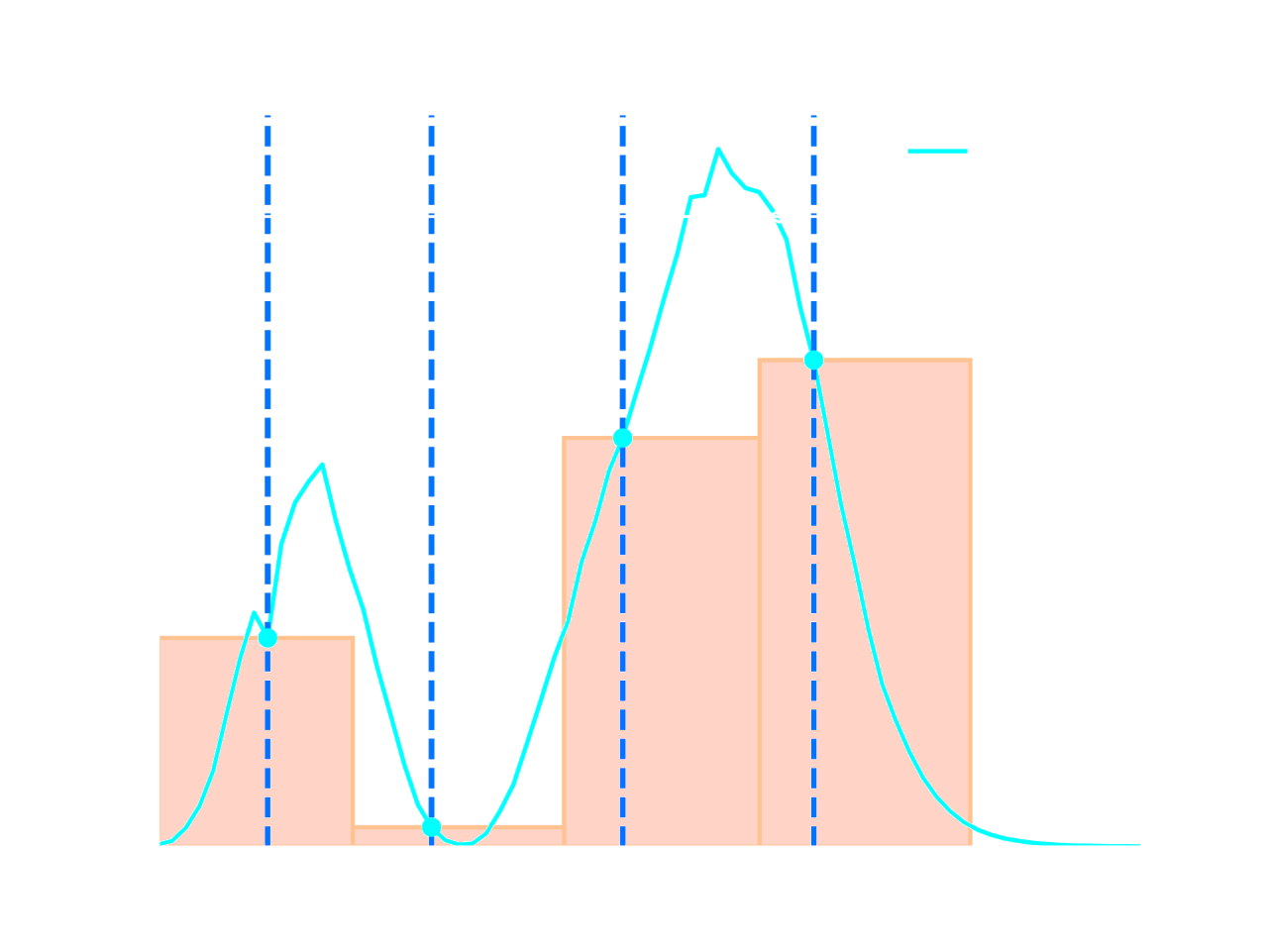 Riemann sum of four partitions, each described by \(\lambda_i\) and \(w_i\). The sum of the areas of all four partitions approximates the integral of \(L(\lambda) \cdot \bar{x}(\lambda)\). The same idea can be applied to the Y and Z values.
The Riemann sum for each tristimulus value can be expressed as:
\[X = \sum_{i=1}^{n_{\lambda}} \bar{x}_i L_i w_i\] \[Y = \sum_{i=1}^{n_{\lambda}} \bar{y}_i L_i w_i\] \[Z = \sum_{i=1}^{n_{\lambda}} \bar{z}_i L_i w_i\]where \(w_i\) is the wavelength interval \(\Delta \lambda\) covered by each partition, which we will call the weight of the partition. Going back to uniform spectral sampling, \(w_i\) is constant in this case as the interval covered by each partition remains constant. In our solution we allow the intervals to change, giving us four more degrees of freedom.
These summations of products can also be written as a matrix multiplication, which is specially useful in order to perform the computations efficiently on the GPU:
\[ \begin{bmatrix} X \\ Y \\ Z \end{bmatrix} = \begin{bmatrix} \bar{x}_1 w_1 & \bar{x}_2 w_2 & \dots & \bar{x}_n w_n \\ \bar{y}_1 w_1 & \bar{y}_2 w_2 & \dots & \bar{y}_n w_n \\ \bar{z}_1 w_1 & \bar{z}_2 w_2 & \dots & \bar{z}_n w_n \end{bmatrix} \begin{bmatrix} L_1 \\ L_2 \\ \vdots \\ L_n \end{bmatrix} \]Optimization
We have seen how using more spectral samples tends to yield a more accurate image, but due to limitations inherent to real-time rendering, we cannot sample dozens of wavelengths like offline renderers do. First, we have to settle for a number of wavelengths to sample.
We have chosen four (\(n_\lambda=4\)) to take advantage of the SIMD instructions available in most modern hardware. The data paths and registers supporting SIMD operations are usually at least 128-bits wide in both CPUs and GPUs, corresponding to four full 32-bit floats. Our algorithm greatly benefits from SIMD vectorization since the light transport simulation is identical for each wavelength; only the data varies.
Four wavelengths might not seem sufficient, but we found that if we choose the best four wavelengths for which to sample \(L(\lambda)\), and the correct weight for each partition \(w_i\), we are able to have all the perks of a spectral renderer with just a single SIMD instruction.
We are left with four partitions, each with a representative wavelength \(\lambda\), and a weight \(w\), totalling eight parameters. The resulting spectrum to tristimulus conversion is:
\[ \begin{bmatrix} X \\ Y \\ Z \end{bmatrix} = \begin{bmatrix} \bar{x}_1 w_1 & \bar{x}_2 w_2 & \bar{x}_3 w_3 & \bar{x}_4 w_4 \\ \bar{y}_1 w_1 & \bar{y}_2 w_2 & \bar{y}_3 w_3 & \bar{y}_4 w_4 \\ \bar{z}_1 w_1 & \bar{z}_2 w_2 & \bar{z}_3 w_3 & \bar{z}_4 w_4 \end{bmatrix} \begin{bmatrix} L(\lambda_1) \\ L(\lambda_2) \\ L(\lambda_3) \\ L(\lambda_4) \end{bmatrix} \]To find the values of the eight parameters that offer the best results when compared to a ground-truth offline simulation, we pose an optimization problem. Mean squared error (MSE) is used as the loss function due its simplicity and adequate results, and is defined as follows:
\[\mathcal{L} = \frac{1}{n} \sum_{\phi,\theta_v,\theta_s} (L_{\phi,\theta_v,\theta_s} - \hat{L}_{\phi,\theta_v,\theta_s})^2\]where \(L_{\phi,\theta_v,\theta_s}\), \(\hat{L}_{\phi,\theta_v,\theta_s}\), are the ground truth and approximated radiance values at a given view direction \((\phi, \theta_v)\) and Sun elevation angle \(\theta_s\), and \(n\) is the total number of combinations of \(\phi\), \(\theta_v\), \(\theta_s\).
This pixel-wise loss function asserts that all view directions and Sun elevation angles are equally important, thus it is important to note that their distribution will affect the optimization. We have deliberately skipped higher Sun elevation angles to put more emphasis on sunrise/sunset conditions, in order to avoid overfitting to the clearly dominant blue color present in daylight.
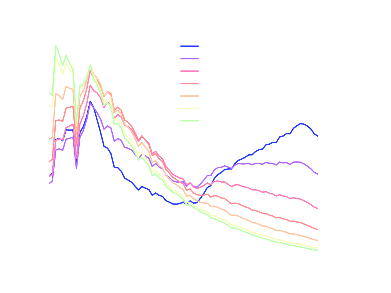 Normalized spectral radiance for several Sun elevations at sea level. The values are averaged across many view directions. Note how long wavelengths (yellows, oranges, reds) become more relevant the lower the Sun elevation angle (sunrise and sunset).
For the optimization process itself, first we performed a brute force grid search of the eight parameters (\(\lambda_1\), \(\lambda_2\), \(\lambda_3\), \(\lambda_4\), \(w_1\), \(w_2\), \(w_3\), \(w_4\)), and then we refined the results using Nelder–Mead.
It is important to note that this optimization only works for a particular atmospheric model. If we optimize for a model, but attempt to use the resulting optimized parameters with another model, the end result will not be correct. In our case, we use the Rayleigh scattering and ozone absorption parts of our atmospheric model, and ignore the aerosols. Aerosols can vary dramatically with the viewer’s position, making them unsuitable for obtaining a general solution to the eight optimization parameters. Luckily for us, they are not as dependent on wavelength as molecules due to their relatively large size, so we found no practical difference between optimizing with and without aerosols.
Rendering and results
During actual real-time rendering we compute the spectral radiance \(L(\lambda)\) for each of the optimized wavelengths (\(\lambda_1\), \(\lambda_2\), \(\lambda_3\), \(\lambda_4\)), and then apply the spectrum to tristimulus conversion. The optimization process we described in the previous section has been performed offline, which means that, at runtime, our method solely requires four spectral samples and a matrix multiplication. Now it is clear why we chose four spectral samples instead of any other number. We can compute \(L(\lambda)\) for the four samples at the same time thanks to SIMD, which makes our method as cheap as traditional RGB rendering.
The end result is a highly accurate render comparable to fully-fledged spectral renderers that require dozens of spectral samples. The image fidelity is also greatly improved in contrast to state to the art algorithms that incorrectly use three spectral radiance values directly as an RGB triplet.
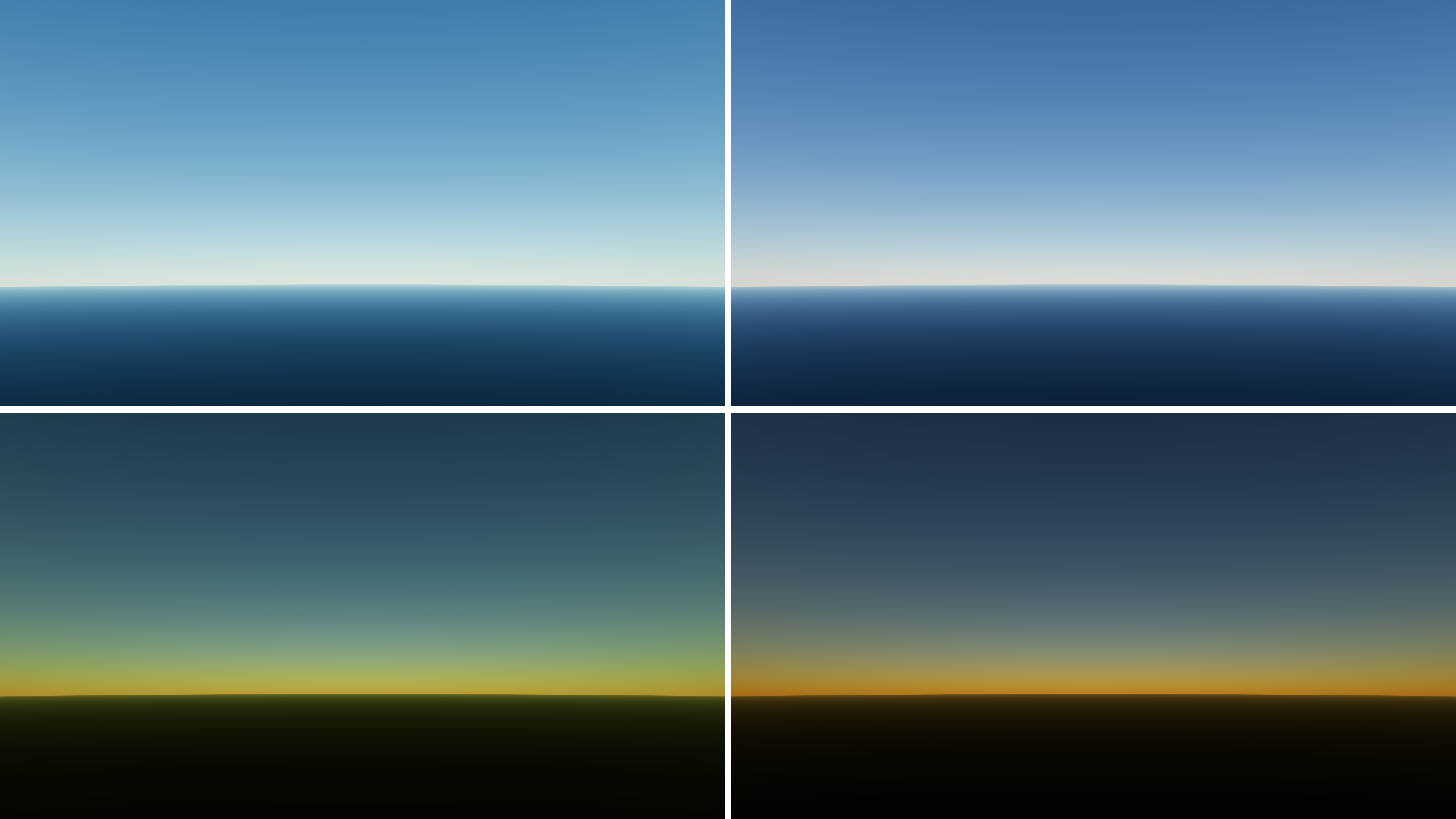 Traditional RGB rendering with 3 wavelengths (680nm, 550nm, 440nm) (left), compared to our spectral rendering method (right). To highlight the differences between both approaches we have removed aerosols as they do not depend on wavelength as much as other constituents.
Conclusion
This technique adds accurate spectral rendering capabilities to any real-time atmosphere rendering framework, like Sébastien Hillaire’s Production Ready Atmosphere or Bruneton’s Precomputed Atmospheric Scattering. It is also not limited to the atmosphere: any participating media which has optical properties that are strongly dependent on wavelength can benefit from this approach, such as human skin and hair, which feature prominent subsurface scattering. All of the methods and the general workflow described above can be applied to these volumetric media.